Wave Simulation

Visualizing the superposition of two-dimensional wave is a kind of challenging. Unlike one-dimensional wave, these wave travels from a point source to all directions around it, which makes it difficult to think about the resulted pattern when there are multiple sources.

One of the typical examples is the interference of two-dimensional waves from 2 point sources. (For the sake of simplicity, the energy dissipation due to increasing length of wavefront is neglected.) According to the text book and observation from experiment, such sources will produce the following interference pattern.

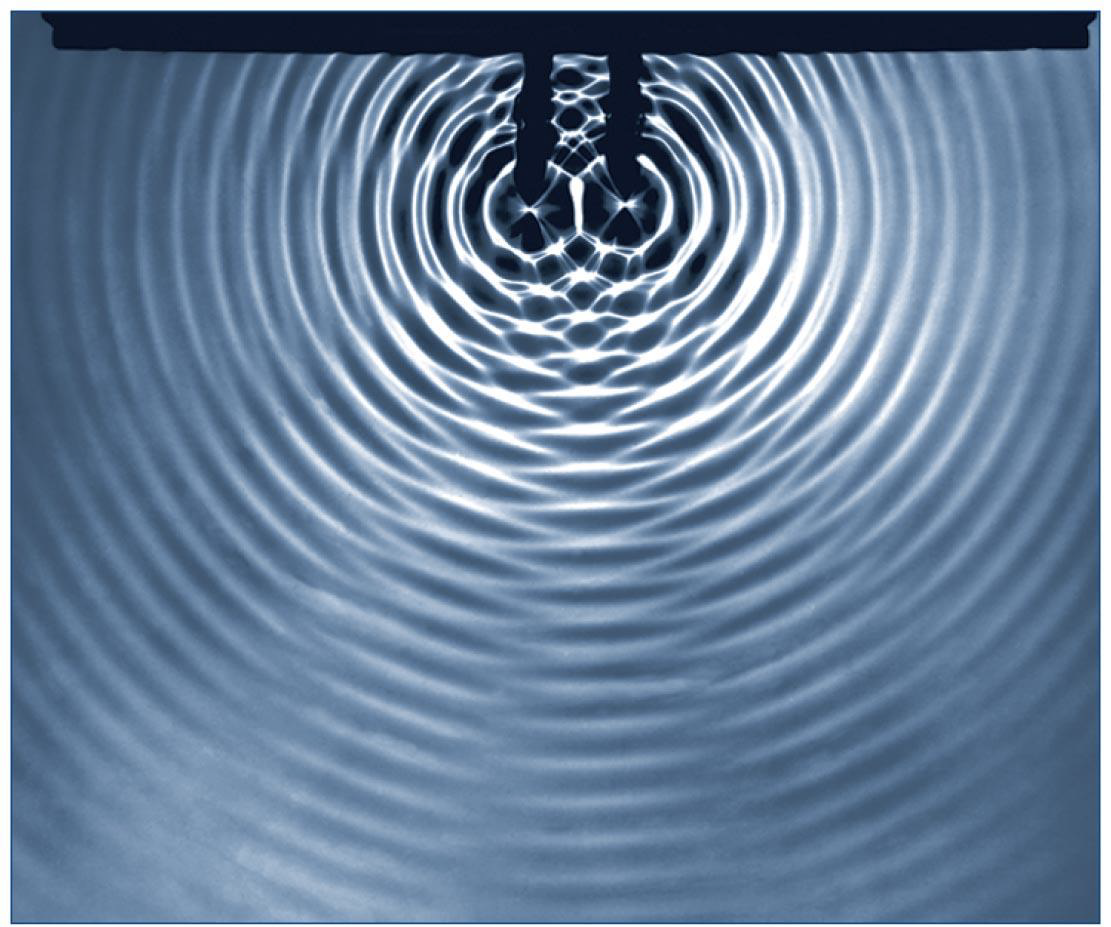
The alternating pattern between fainter and darker areas are the result of destructive and constructive interference. In fact, because these patterns form lines extending from roughly the center of the two sources and propagate outward. They are called nodal lines and antinodal lines. But why are these lines where they are? And how many of them should present? To answer these questions, I decided to make a simulation to see if I can reproduce them.

Wave Equation

At first, I thought it would be good to start with wave equation.

$$\frac{\partial f}{\partial x} = \frac{1}{c^2} \frac{\partial f}{\partial t}$$

However, this does not seems to be a good idea as I will need to solve the partial differential equation to get the explicit wave function $f$, which may be over complicated for this task. (There might be ways to build simulations with only differential equations, but I am not very familiar with those methods).

Wave Function

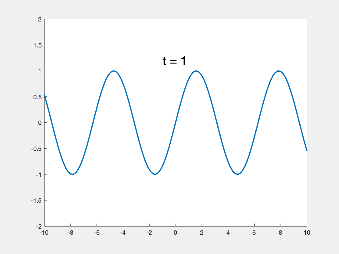
A much easier approach will be to use the wave function, or the explicit form of $f$ that satisfied the above equation. From the textbook, the time-dependent wave function for one dimensional wave is given in the following form:

$$f(x, t) = g(x-ct+\phi)$$

In this function, $x$ represents the position and $t$ represents time, the function $f$ represents the amplitude of the wave at given time and position, and function $g$ determines the shape of the wave. The constant $c$ represents the wavespeed, and constant $\phi$ represents the initial phase. For example, if we plugin $g = \sin(x)$ and $\phi=0$. The function $f(x,t) = sin(x-ct+\phi)$ describes a traveling sinusoidal wave.

With this scheme, the wave function for two dimensional waves can be derived by changing the position $x$ into the distance between a position and the wave source.

$$f(x, y, t) = \sin(\sqrt{(x-x_0)^2 + (y-y_0)^2} - ct + \phi)$$

Great! With this wave function, we can finally create the simulation by computing the amplitude at all points on a plane over some period of time. When there are more than one wave source, the amplitude of a given point on the plane is the sum of the amplitude of the wave from every source. After tuning some parameters for presentation, the final result looks like this.

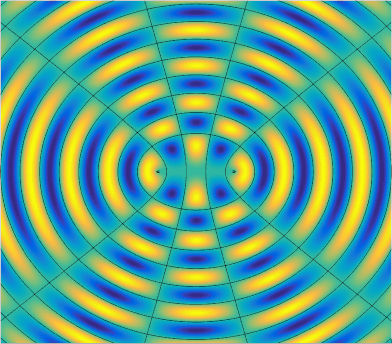
The black lines and circles represents zero amplitude at a given time. Notice that the black lines that does not change with respect to time is the nodal line, which has a path length difference (the difference of the distance to two point source) of some odd integer multiples of half wavelength, or $\delta s = \frac{m}{2}\lambda, m = 1, 3, 5, ...$

One interesting fact of the interference pattern of two point sources is that the number of (anti)nodal lines depend only on the source separation $d$. In this animation, $d = 2\lambda$. You can figure this out by marking the path length difference $\delta$ of (anti)nodal lines from the perpendicular bisector ($\delta=0$) to the horizontal line connecting the two sources ($\delta=d=2\lambda$), with each adjacent (anti)nodal line increases $\delta$ by $\frac{1}{2}\lambda$.

Perfecting the model

To create a more accurate model, I need to take the energy dissipation into account, as the resulting wavefront in simulation apparently increases its intensity as it propagates, which is not observed in the experiment.

To compute the energy dissipation, the energy per unit length of wavefront is in inverse proportion to the distance traveled, or the radius, as the total energy of wave pulse conserved. Because energy is in direct proportion to the square of amplitude. the resulting adjustment looks like this ($k$ is some constant):

$$f(x, y, t) = \frac{k}{\sqrt[4]{(x-x_0)^2 + (y-y_0)^2}}\cdot\sin(\sqrt{(x-x_0)^2 + (y-y_0)^2} - ct + \phi)$$

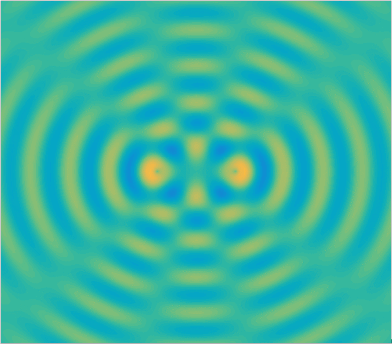
After adjustment, the (anti)nodal lines get fuzzier when they spread out, which is similar to what happened in the reality comparing to the photo in the beginning. I hide the contour plot because they no longer form a clear pattern as before. Because of the way it is adjusted, the amplitude at the point source will approach infinity (the denominator approaches zero). This is where the simulation falls short (notice the point source is extremely bright), and I am not sure how to fix it, so feel free to let me know if you have better ideas.

Huygens Principle

With the simulation framework we had, we can do more than the typical two source interference. For example, we can visualize Huygens Principle by placing many tightly spaced point sources in a line. This is the model for plane wave.

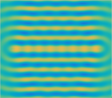
This simulation uses 101 point sources in a line, and the result resembles a plane wave as expected. Of course I cannot simulate infinitely many point sources, but you get the idea. Notice the wavefront has relatively low amplitude around the horizontal direction at each end of the “line” of wave sources due to the lack of interference.

The code for this simulation is released in Github, feel free to play with it.